Background
Locating an epicentre with the circle method needs at least three seismic stations. From each station we need the arrival times of the P and S waves, whose difference gives the S-P time. The S-P time is used to estimate the distance travelled; in this example we use the Tau-P method for that. The method is also called circle and chord, because it uses the intersections of the circles and the lines (chords) through those intersections.
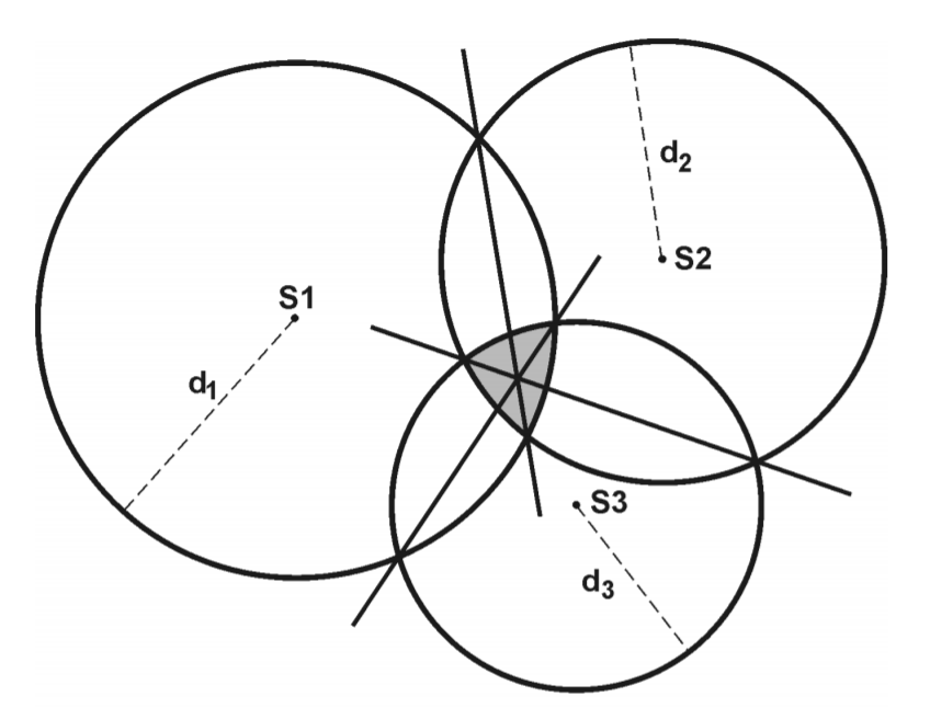
In the figure above (Havskov et al., 2002), S is a seismic station and d is the distance obtained by matching the S-P time to a distance.
Data
We use the P and S arrival times of the M6.2 Mamuju earthquake recorded at the stations TATO (Taiwan), PMG (Port Moresby) and COCO (Cocos Island). The arrival times are converted to the obspy UTCDateTime format:
from obspy import UTCDateTime

TATO_P = UTCDateTime("2021-01-14T18:34:08")
TATO_S = UTCDateTime("2021-01-14T18:38:53")

PMG_P = UTCDateTime("2021-01-14T18:34:15")
PMG_S = UTCDateTime("2021-01-14T18:39:04")

COCO_P = UTCDateTime("2021-01-14T18:33:28")
COCO_S = UTCDateTime("2021-01-14T18:37:43")
Difference between S and P arrival times
The S-P difference is computed simply as:
TATO_SP = TATO_S-TATO_P
PMG_SP = PMG_S-PMG_P
COCO_SP = COCO_S-COCO_P

print(COCO_SP,"sekon")
255.0 sekon
Estimating the distance with a rule of thumb
From the S-P value we can directly estimate the circle radius (distance) with the formula of Havskov et al. (2002):
$$distance=(SP-2)\times10,$$
in kilometres. To convert it to degrees, we divide by 111.26 km:
jarak=[(SP-2)*10/111.26 for SP in [TATO_SP,PMG_SP,COCO_SP]]
jarak
[25.43591587273054, 25.795434118281502, 22.73952903109833]
Then we can plot it:
import matplotlib.pyplot as plt

# station coordinates
TATO_coor=(121.50,24.97)
PMG_coor=(147.16,-9.40)
COCO_coor=(96.83,-12.19)

nama_stasiun = ["TATO","PMG","COCO"]

figure, ax = plt.subplots()

ax.set_aspect(1)
for sta,rad,nsta in zip([TATO_coor, PMG_coor, COCO_coor],\
               jarak,nama_stasiun):
    ax.scatter(sta[0],sta[1], zorder=100, marker="v", color="blue")
    draw_circle =plt.Circle(sta, rad, fill=False)
    ax.add_artist(draw_circle)
    ax.annotate(nsta, sta)


ax.set_title('Episenter Metode Lingkaran Gempa Mamuju M6,2')
ax.set_xlim(70,180)
ax.set_ylim(-40,60)
ax.scatter(118.8893,-2.9711,color="red", label="Episenter sebenarnya (IRIS)")
ax.legend()
plt.show()

This approximation is reasonable but not accurate. We can improve the accuracy with Tau-P.
Finding the distance from S-P
Introducing the TauPyModel module from obspy
Before finding the distance from S-P, we get to know the TauPyModel module from obspy. It computes the travel time from an earthquake to a station for a given location and depth. The module is based on the Tau-P algorithm and works with several existing velocity models; we use IASP91. Besides travel times, it can also plot the raypaths:
from obspy.taup import TauPyModel
model = TauPyModel(model="iasp91")

#example: travel time for an earthquake at 60 km depth and an epicentral distance of 60 degrees
arrivals = model.get_travel_times(source_depth_in_km=60, #depth in km
                                      distance_in_degree=60)# jarak dalam derajat

print(arrivals)
26 arrivals
	P phase arrival at 600.258 seconds
	pP phase arrival at 616.298 seconds
	sP phase arrival at 623.358 seconds
	PcP phase arrival at 645.616 seconds
	PP phase arrival at 733.120 seconds
	ScP phase arrival at 881.182 seconds
	PcS phase arrival at 888.006 seconds
	PKiKP phase arrival at 1024.399 seconds
	pPKiKP phase arrival at 1042.077 seconds
	sPKiKP phase arrival at 1048.763 seconds
	S phase arrival at 1088.878 seconds
	SP phase arrival at 1100.115 seconds
	pS phase arrival at 1107.826 seconds
	PS phase arrival at 1109.778 seconds
	sS phase arrival at 1116.576 seconds
	ScS phase arrival at 1185.125 seconds
	SKiKP phase arrival at 1231.805 seconds
	SS phase arrival at 1327.584 seconds
	PKIKKIKP phase arrival at 1864.119 seconds
	SKIKKIKP phase arrival at 2071.513 seconds
	PKIKKIKS phase arrival at 2078.199 seconds
	SKIKKIKS phase arrival at 2285.426 seconds
	PKIKPPKIKP phase arrival at 2364.644 seconds
	PKPPKP phase arrival at 2375.132 seconds
	PKPPKP phase arrival at 2386.588 seconds
	SKIKSSKIKS phase arrival at 3216.623 seconds
To plot them, we use get_raypaths:
raypaths = model.get_ray_paths(source_depth_in_km=60, #depth in km
                                      distance_in_degree=60)# jarak dalam derajat

ax = raypaths.plot_rays()

We can also restrict which phases are computed with the phase_list parameter:
arrivals = model.get_travel_times(source_depth_in_km=60, #depth in km
                                      distance_in_degree=60,# jarak dalam derajat
                                     phase_list=["P","S"])#daftar fase yang akan diambil

print(arrivals)
2 arrivals
	P phase arrival at 600.258 seconds
	S phase arrival at 1088.878 seconds
raypaths = model.get_ray_paths(source_depth_in_km=60, #depth in km
                               distance_in_degree=60, # distance in degrees
                              phase_list=["P","S"])#daftar fase yang akan diambil

ax = raypaths.plot_rays()

To get the arrival times as numbers, we use indexing and the .time and .name attributes. For example, the first arrival:
first_arrival=arrivals[0]
nama_fase=first_arrival.name
waktu_tiba=first_arrival.time

print("Fase pertama datang {} pada {} sekon".format(nama_fase, waktu_tiba))
Fase pertama datang P pada 600.2579575887129 sekon
The P arrival clearly comes first, so we use index 0 as above. The S arrival needs a small modification, because a single event can have several P and S phases, for example:
arrivals = model.get_travel_times(source_depth_in_km=10,
                                      distance_in_degree=23.6,
                                      phase_list=["P","S"])
print(arrivals)
8 arrivals
	P phase arrival at 311.128 seconds
	P phase arrival at 311.211 seconds
	P phase arrival at 312.946 seconds
	S phase arrival at 566.326 seconds
	S phase arrival at 568.932 seconds
	S phase arrival at 571.185 seconds
	S phase arrival at 586.578 seconds
	S phase arrival at 586.600 seconds
The example above has three P arrivals and five S arrivals. How do we pick the first S arrival? We can write a small algorithm:
Collect the phase names in a loop:
import numpy as np
phase_names=np.array([arr.name for arr in arrivals])
phase_names
array(['P', 'P', 'P', 'S', 'S', 'S', 'S', 'S'],
      dtype='<U1')
Find the indices of the S phases:
S_indexes=np.where(phase_names=="S")
S_indexes
(array([3, 4, 5, 6, 7]),)
Take the first S index as the index of the first S arrival:
S_index=S_indexes[0][0]
S_index
3
Use that index to get the first S arrival:
Sfirst_arrival=arrivals[S_index]
Snama_fase=Sfirst_arrival.name
Swaktu_tiba=Sfirst_arrival.time

print("Fase S pertama datang {} pada {} sekon".format(Snama_fase, Swaktu_tiba))
Fase S pertama datang S pada 566.3255616737924 sekon
Using TauPyModel to find the distance
As discussed above, TauPyModel computes wave travel times. The circle method needs the opposite: from travel time to distance. So we write a short piece of code that inverts the procedure; here the depth is fixed at 10 km.
Next, we try each distance with a for loop and compute the S-P value from TauPyModel: SP_taup=arrivals[-1].time-arrivals[0].time. A condition below this step says: if the S-P time from TauPyModel is smaller than the observed S-P time at the station, that distance is accepted; if it is larger, the distance is not updated.
As an illustration, suppose we want to guess the distance for an S-P time of 250 s and a depth of 10 km, trying distances from 22 to 25 degrees in steps of 1:
distance_list=np.arange(22,25,1) #range of guesses
SP=250 #SP (s)
depth=10 #km

initial_distance=distance_list[0]
for dist in distance_list:
    arrivals = model.get_travel_times(source_depth_in_km=depth,
                                      distance_in_degree=dist,
                                      phase_list=["P","S"])
    # the P arrival is always the first
    P_arrival = arrivals[0].time

    # careful with the S arrival, there can be several P and S phases
    phase_names=np.array([arr.name for arr in arrivals]) # collect the phase names
    S_indexes=np.where(phase_names=="S") #indices of the S phases
    S_index=S_indexes[0][0] # index of the first S phase
    S_arrival = arrivals[S_index].time # S arrival time

    # compute S-P from TauP IASP91
    SP_taup = S_arrival-P_arrival

    if SP_taup<SP: #if SP_taup < observed SP, update the distance
        print("SP taup < SP: {} < {}".format(SP_taup,SP))
        print("Initial distance diupdate: {}".format(initial_distance))
        initial_distance = dist
    else: # otherwise the distance is not updated
        print("SP taup > SP: {} > {}".format(SP_taup,SP))
        print("Initial distance tidak diupdate: {}".format(initial_distance))


print("Jarak yang terpilih: {}".format(initial_distance))
SP taup < SP: 243.80686273283436 < 250
Initial distance diupdate: 22
SP taup > SP: 251.6500605586528 > 250
Initial distance tidak diupdate: 22
SP taup > SP: 258.02310930613214 > 250
Initial distance tidak diupdate: 22
Jarak yang terpilih: 22
The example above selects a distance of 22 degrees, because its S-P value (243 s) is smaller than the observed 250 s. At 23 degrees the value (251 s) is already larger than 250 s, so 23 degrees and beyond are rejected. This algorithm has a weakness: although S-P > 250 s at 23 degrees, the difference is only about 1.65 s, much smaller than the 6.2 s difference at 22 degrees. We therefore add a new condition:
distance_list=np.arange(22,25,1)
SP=250
depth=10 #km

initial_distance=distance_list[0]

for dist in distance_list:
    arrivals = model.get_travel_times(source_depth_in_km=depth,
                                      distance_in_degree=dist,
                                      phase_list=["P","S"])
    P_arrival = arrivals[0].time

    # careful with the S arrival, there can be several P and S phases
    phase_names=np.array([arr.name for arr in arrivals]) # collect the phase names
    S_indexes=np.where(phase_names=="S") #indices of the S phases
    S_index=S_indexes[0][0] # index of the first S phase
    S_arrival = arrivals[S_index].time # S arrival time

    SP_taup = S_arrival-P_arrival

    if SP_taup<SP:
        initial_distance = dist
        print("SP taup < SP: {} < {}".format(SP_taup,SP))
        print("Initial distance diupdate: {}".format(initial_distance))
        SP_error=abs(SP_taup-SP) #add the SP_error calculation

    else:
        SP_error_check = abs(SP_taup-SP)
        if SP_error_check < SP_error: # if the current SP_error < the previous SP_error, still update the distance
            print("SP taup > SP: {} > {}".format(SP_taup,SP))
            print("Tetapi SP_error < SP_error_sebelumnya: {} < {}".format(SP_error_check, SP_error))
            initial_distance = dist
            print("Initial distance diupdate: {}".format(initial_distance))

        else:
            print("SP taup > SP: {} > {}".format(SP_taup,SP))
            print("Initial distance tidak diupdate: {}".format(initial_distance))


print("Jarak yang terpilih: {}".format(initial_distance))
SP taup < SP: 243.80686273283436 < 250
Initial distance diupdate: 22
SP taup > SP: 251.6500605586528 > 250
Tetapi SP_error < SP_error_sebelumnya: 1.6500605586527968 < 6.193137267165639
Initial distance diupdate: 23
SP taup > SP: 258.02310930613214 > 250
Initial distance tidak diupdate: 23
Jarak yang terpilih: 23
We now get the distance whose S-P value is closer to the observation: 23 degrees.
Choosing the range of distance guesses
We can match S-P against a travel-time curve, but first we convert S-P to minutes:
print(TATO_SP/60, PMG_SP/60, COCO_SP/60)
4.75 4.816666666666666 4.25
With Tau-P we can draw a travel-time curve:
from obspy.taup import plot_travel_times
import matplotlib.pyplot as plt

fig, ax = plt.subplots(figsize=(6, 6))
ax = plot_travel_times(source_depth=10, phase_list=["P", "S"],
                       ax=ax, fig=fig, verbose=True,
                      show=False)
ax.set_title("Kurva Waktu Tempuh P S untuk Kedalaman 10 km")
ax.grid()
There were 23 epicentral distances without an arrival

Our S-P values range from 4.25 to 4.8 minutes, so based on the curve above we zoom in on 10 to 40 degrees:
fig, ax = plt.subplots(figsize=(6, 6))
ax = plot_travel_times(source_depth=10, phase_list=["P", "S"],
                       ax=ax, fig=fig, verbose=True, min_degrees=10, max_degrees=40, #zoom
                      show=False)
ax.set_title("Kurva Waktu Tempuh P S untuk Kedalaman 10 km")
ax.grid()
There were 0 epicentral distances without an arrival

From the zoomed curve we choose a guess range of 20 to 30 degrees.
Finding the correct station-earthquake distance
To find the right distance for each station, we add one more for loop and search from 20 to 30 degrees in finer steps of 0.1:
distance_list=np.arange(20,30,0.1)
station_SP_list=[TATO_SP,PMG_SP,COCO_SP]

sta_distance_list=[]
for sta_SP in station_SP_list:
    initial_distance=distance_list[0]
    for dist in distance_list:
        arrivals = model.get_travel_times(source_depth_in_km=depth,
                                          distance_in_degree=dist,
                                          phase_list=["P","S"])
        P_arrival = arrivals[0].time

        # careful with the S arrival, there can be several P and S phases
        phase_names=np.array([arr.name for arr in arrivals]) # collect the phase names
        S_indexes=np.where(phase_names=="S") #indices of the S phases
        S_index=S_indexes[0][0] # index of the first S phase
        S_arrival = arrivals[S_index].time # S arrival time

        SP_taup = S_arrival-P_arrival

        if SP_taup<sta_SP:
            initial_distance = dist
            SP_error=abs(SP_taup-sta_SP) #add the SP_error calculation

        else:
            SP_error_check = abs(SP_taup-sta_SP)
            if SP_error_check < SP_error: # if the current SP_error < the previous SP_error, still update the distance
                initial_distance = dist

    sta_distance_list.append(initial_distance)
sta_distance_list
[27.900000000000112, 28.500000000000121, 23.50000000000005]
With this algorithm we get distances of 27.9, 28.5 and 23.5 degrees for TATO, PMG and COCO.
Plotting the result with matplotlib
The circles can be plotted with plt.Circle, using the station coordinates as centres and the distances found above as radii:
import matplotlib.pyplot as plt

# station coordinates
TATO_coor=(121.50,24.97)
PMG_coor=(147.16,-9.40)
COCO_coor=(96.83,-12.19)
#list of station names
nama_stasiun = ["TATO","PMG","COCO"]

figure, ax = plt.subplots()

ax.set_aspect(1) #keep the x and y proportions equal

# plot circles and points
for sta,rad,nsta in zip([TATO_coor, PMG_coor, COCO_coor],\
               sta_distance_list,nama_stasiun):
    ax.scatter(sta[0],sta[1], zorder=100, marker="v", color="blue") #station points
    draw_circle =plt.Circle(sta, rad, fill=False) #circle
    ax.add_artist(draw_circle) #circle
    ax.annotate(nsta, sta) # station names


ax.set_title('Episenter Metode Lingkaran Gempa Mamuju M6,2')
ax.set_xlim(70,180)
ax.set_ylim(-40,60)
ax.scatter(118.8893,-2.9711,color="red", label="Episenter sebenarnya (IRIS)")
ax.legend()
plt.show()

Plotting the result with cartopy
import numpy as np
import cartopy.crs as ccrs
from cartopy.io import srtm
import matplotlib.pyplot as plt
import cartopy.io.img_tiles as cimgt

fig = plt.figure()
ax = plt.axes(projection=ccrs.PlateCarree())
ax.set_extent((70,180,-40,60))

# Add stamen background
stamen_terrain = cimgt.Stamen('terrain-background') ##maps.stamen.com
ax.add_image(stamen_terrain,2)

ax.set_xlabel("Longitude [deg]")
ax.set_ylabel("Latitude [deg]")

gl = ax.gridlines(draw_labels=True, dms=False, x_inline=False, y_inline=False, zorder=11)

gl.xlabels_top = False
gl.ylabels_right = False

for sta,rad,nsta in zip([TATO_coor, PMG_coor, COCO_coor],\
               sta_distance_list,nama_stasiun):
    ax.scatter(sta[0],sta[1], zorder=100, marker="v", color="blue")
    draw_circle =plt.Circle(sta, rad, fill=False)
    ax.add_artist(draw_circle)
    ax.annotate(nsta, sta)


ax.scatter(118.8893,-2.9711,color="red", label="Episenter sebenarnya (IRIS)")

plt.savefig("output/demo_epi.png",dpi=300)
/home/anangsahroni/Environments/envgeneral/lib/python3.9/site-packages/cartopy/mpl/gridliner.py:324: UserWarning: The .xlabels_top attribute is deprecated. Please use .top_labels to toggle visibility instead.
  warnings.warn('The .xlabels_top attribute is deprecated. Please '
/home/anangsahroni/Environments/envgeneral/lib/python3.9/site-packages/cartopy/mpl/gridliner.py:360: UserWarning: The .ylabels_right attribute is deprecated. Please use .right_labels to toggle visibility instead.
  warnings.warn('The .ylabels_right attribute is deprecated. Please '

Code summary
Combining the code above into one block gives:
import numpy as np
from obspy import UTCDateTime
import cartopy.crs as ccrs
import matplotlib.pyplot as plt
import cartopy.io.img_tiles as cimgt
from obspy.taup import TauPyModel

# VELOCITY MODEL
model = TauPyModel(model="iasp91")

# DEPTH
depth=10 #km

# DATA
TATO_P = UTCDateTime("2021-01-14T18:34:08")
TATO_S = UTCDateTime("2021-01-14T18:38:53")

PMG_P = UTCDateTime("2021-01-14T18:34:15")
PMG_S = UTCDateTime("2021-01-14T18:39:04")

COCO_P = UTCDateTime("2021-01-14T18:33:28")
COCO_S = UTCDateTime("2021-01-14T18:37:43")

# COORDINATES and NAMES
TATO_coor=(121.50,24.97)
PMG_coor=(147.16,-9.40)
COCO_coor=(96.83,-12.19)
nama_stasiun = ["TATO","PMG","COCO"]

# SP
TATO_SP = TATO_S-TATO_P
PMG_SP = PMG_S-PMG_P
COCO_SP = COCO_S-COCO_P

# FIND THE DISTANCE
distance_list=np.arange(20,30,0.1) #Range of guesses
station_SP_list=[TATO_SP,PMG_SP,COCO_SP]

sta_distance_list=[]
for sta_SP in station_SP_list:
    initial_distance=distance_list[0]
    for dist in distance_list:
        arrivals = model.get_travel_times(source_depth_in_km=depth,
                                          distance_in_degree=dist,
                                          phase_list=["P","S"])
        P_arrival = arrivals[0].time

        # careful with the S arrival, there can be several P and S phases
        phase_names=np.array([arr.name for arr in arrivals]) # collect the phase names
        S_indexes=np.where(phase_names=="S") #indices of the S phases
        S_index=S_indexes[0][0] # index of the first S phase
        S_arrival = arrivals[S_index].time # S arrival time

        SP_taup = S_arrival-P_arrival

        if SP_taup<sta_SP:
            initial_distance = dist
            SP_error=abs(SP_taup-sta_SP) #add the SP_error calculation

        else:
            SP_error_check = abs(SP_taup-sta_SP)
            if SP_error_check < SP_error: # if the current SP_error < the previous SP_error, still update the distance
                initial_distance = dist

    sta_distance_list.append(initial_distance)


# PLOT
fig = plt.figure()
ax = plt.axes(projection=ccrs.PlateCarree())
ax.set_extent((70,180,-40,60))

# Add stamen background
stamen_terrain = cimgt.Stamen('terrain-background') ##maps.stamen.com
ax.add_image(stamen_terrain,2) # 2 is the zoom level: higher means more detail but a longer download, use it wisely

ax.set_xlabel("Longitude [deg]")
ax.set_ylabel("Latitude [deg]")

gl = ax.gridlines(draw_labels=True, dms=False, x_inline=False, y_inline=False, zorder=11)

gl.xlabels_top = False
gl.ylabels_right = False

for sta,rad,nsta in zip([TATO_coor, PMG_coor, COCO_coor],\
               sta_distance_list,nama_stasiun):
    ax.scatter(sta[0],sta[1], zorder=100, marker="v", color="blue")
    draw_circle =plt.Circle(sta, rad, fill=False)
    ax.add_artist(draw_circle)
    ax.annotate(nsta, sta)


ax.scatter(118.8893,-2.9711,color="red", label="Episenter sebenarnya (IRIS)")

plt.savefig("output/demo_epi.png",dpi=300)
/home/anangsahroni/Environments/envgeneral/lib/python3.9/site-packages/cartopy/mpl/gridliner.py:324: UserWarning: The .xlabels_top attribute is deprecated. Please use .top_labels to toggle visibility instead.
  warnings.warn('The .xlabels_top attribute is deprecated. Please '
/home/anangsahroni/Environments/envgeneral/lib/python3.9/site-packages/cartopy/mpl/gridliner.py:360: UserWarning: The .ylabels_right attribute is deprecated. Please use .right_labels to toggle visibility instead.
  warnings.warn('The .ylabels_right attribute is deprecated. Please '

Extra: finding the epicentre point
Simplifying the problem to a flat plane, we can use geometry to find the two intersection points of two circles:
# reference: https://stackoverflow.com/questions/64800285/intersection-coordinates-lat-lon-of-two-circles-given-the-coordinates-of-the
import math
def circle_intersection(x0, y0, r0, x1, y1, r1):

    d = math.sqrt((x1 - x0) ** 2 + (y1 - y0) ** 2)

    if d > r0 + r1:             # non intersecting
        return None
    if d < abs(r0 - r1):        # one circle within other
        return None
    if d == 0 and r0 == r1:     # coincident circles
        return None

    a = (r0 ** 2 - r1 ** 2 + d ** 2) / (2 * d)
    h = math.sqrt(r0 ** 2 - a ** 2)
    x2 = x0 + a * (x1 - x0) / d
    y2 = y0 + a * (y1 - y0) / d
    x3 = x2 + h * (y1 - y0) / d
    y3 = y2 - h * (x1 - x0) / d

    x4 = x2 - h * (y1 - y0) / d
    y4 = y2 + h * (x1 - x0) / d

    return (x3, y3), (x4, y4)
We use the function above to compute the intersections of each pair of station circles:
TP_1, TP_2 = circle_intersection(TATO_coor[0], TATO_coor[1], sta_distance_list[0],\
                   PMG_coor[0], PMG_coor[1], sta_distance_list[1])

TC_1, TC_2 = circle_intersection(TATO_coor[0], TATO_coor[1], sta_distance_list[0],\
                   COCO_coor[0], COCO_coor[1], sta_distance_list[2])

PC_1, PC_2 = circle_intersection(PMG_coor[0], PMG_coor[1], sta_distance_list[1],\
                   COCO_coor[0], COCO_coor[1], sta_distance_list[2])

print(TP_1, TP_2)
(119.42228880002661, -2.852528931955689) (148.76572171237126, 19.054729972052563)
Then we convert the result to a list for convenience:
#TATO PMG
TPx=[TP_1[0], TP_2[0]]
TPy=[TP_1[1], TP_2[1]]

#TATO COCO
TCx=[TC_1[0], TC_2[0]]
TCy=[TC_1[1], TC_2[1]]

# PMG_COCO
PCx=[PC_1[0], PC_2[0]]
PCy=[PC_1[1], PC_2[1]]
With two intersection points per pair, we can plot the chord lines:
import matplotlib.pyplot as plt

# station coordinates
TATO_coor=(121.50,24.97)
PMG_coor=(147.16,-9.40)
COCO_coor=(96.83,-12.19)

nama_stasiun = ["TATO","PMG","COCO"]

figure, ax = plt.subplots()

ax.set_aspect(1)
for sta,rad,nsta in zip([TATO_coor, PMG_coor, COCO_coor],\
               sta_distance_list,nama_stasiun):
    ax.scatter(sta[0],sta[1], zorder=100, marker="v", color="blue")
    draw_circle =plt.Circle(sta, rad, fill=False)
    ax.add_artist(draw_circle)
    ax.annotate(nsta, sta)

# plot the chord lines
ax.plot(TPx, TPy)
ax.plot(TCx, TCy)
ax.plot(PCx, PCy)

ax.set_title('Episenter Metode Lingkaran Gempa Mamuju M6,2')
ax.set_xlim(70,180)
ax.set_ylim(-40,60)
ax.scatter(118.8893,-2.9711,color="red", label="Episenter sebenarnya (IRIS)")
ax.legend()
plt.show()

With linregress from scipy we easily get the slope and intercept of each chord line:
from scipy import stats
result = stats.linregress(TPx, TPy)
mTP=result.slope
cTP=result.intercept

result = stats.linregress(TCx, TCy)
mTC=result.slope
cTC=result.intercept

result = stats.linregress(PCx, PCy)
mPC=result.slope
cPC=result.intercept
A simple equation gives the intersection of two lines:
def two_intersection(m1,c1,m2,c2):
    x=(c2-c1)/(m1-m2)
    y=m1*x+c1
    return x,y
The intersection of each pair is computed and then averaged:
inter_TPPC=two_intersection(mTP, cTP, mPC, cPC)
inter_TPTC=two_intersection(mTP, cTP, mTC, cTC)
inter_PCTC=two_intersection(mPC, cPC, mTC, cTC)

print(inter_TPPC)
print(inter_TPTC)
print(inter_PCTC)
(118.98966796026603, -3.175515569961405)
(118.98966796026605, -3.1755155699613908)
(118.98966796026603, -3.175515569961135)
The intersection points of the pairs differ only in the 12th decimal place, so a simple average is enough:
x_av=(inter_TPPC[0]+inter_TPTC[0]+inter_PCTC[0])/3
y_av=(inter_TPPC[1]+inter_TPTC[1]+inter_PCTC[1])/3

print("Episenter hasil kalkulasi",x_av, y_av)
print("Episenter sebenarnya: 118.8893,-2.9711")
Episenter hasil kalkulasi 118.98966796 -3.17551556996
Episenter sebenarnya: 118.8893,-2.9711
We plot it and zoom in to see it better:
import matplotlib.pyplot as plt

# station coordinates
TATO_coor=(121.50,24.97)
PMG_coor=(147.16,-9.40)
COCO_coor=(96.83,-12.19)

nama_stasiun = ["TATO","PMG","COCO"]

figure, ax = plt.subplots()

ax.set_aspect(1)
for sta,rad,nsta in zip([TATO_coor, PMG_coor, COCO_coor],\
               sta_distance_list,nama_stasiun):
    ax.scatter(sta[0],sta[1], zorder=100, marker="v", color="blue")
    draw_circle =plt.Circle(sta, rad, fill=False)
    ax.add_artist(draw_circle)
    ax.annotate(nsta, sta)

ax.plot(TPx, TPy)
ax.plot(TCx, TCy)
ax.plot(PCx, PCy)

ax.set_title('Episenter Metode Lingkaran Gempa Mamuju M6,2')
ax.set_xlim(115,125)
ax.set_ylim(-5,2)
ax.scatter(118.8893,-2.9711,color="red", label="Episenter sebenarnya (IRIS)")
ax.scatter(x_av,y_av,color="green", label="Episenter kalkulasi")
ax.legend()
plt.show()

fig = plt.figure()
ax = plt.axes(projection=ccrs.PlateCarree())
ax.set_extent((115,125,-6,1))

# Add custom background
terrain = cimgt.GoogleTiles(url='https://server.arcgisonline.com/ArcGIS/rest/services/World_Shaded_Relief/MapServer/tile/{z}/{y}/{x}.jpg',\
                           cache=True)
ax.add_image(terrain,8) # 8 is the zoom level of the basemap,
                    #higher means more detail but a longer download, use it wisely

ax.set_xlabel("Longitude [deg]")
ax.set_ylabel("Latitude [deg]")

gl = ax.gridlines(draw_labels=True, dms=False, x_inline=False, y_inline=False, zorder=1)

gl.xlabels_top = False
gl.ylabels_right = False

for sta,rad,nsta in zip([TATO_coor, PMG_coor, COCO_coor],\
               sta_distance_list,nama_stasiun):
    ax.scatter(sta[0],sta[1], zorder=100, marker="v", color="blue")
    draw_circle =plt.Circle(sta, rad, fill=False)
    ax.add_artist(draw_circle)
    ax.annotate(nsta, sta)

ax.plot(TPx, TPy)
ax.plot(TCx, TCy)
ax.plot(PCx, PCy)

ax.scatter(118.8893,-2.9711,color="red", label="Episenter sebenarnya (IRIS)")
ax.scatter(x_av,y_av,color="green", label="Episenter kalkulasi")

ax.legend()
plt.savefig("output/demo_epi_pt.png",dpi=300)

Extended summary
The code summary extended with the algorithm for finding the point:
import math
import numpy as np
from scipy import stats
from obspy import UTCDateTime
import cartopy.crs as ccrs
import matplotlib.pyplot as plt
import cartopy.io.img_tiles as cimgt
from obspy.taup import TauPyModel

# VELOCITY MODEL
model = TauPyModel(model="iasp91")

# DEPTH
depth=10 #km

# DATA
TATO_P = UTCDateTime("2021-01-14T18:34:08")
TATO_S = UTCDateTime("2021-01-14T18:38:53")

PMG_P = UTCDateTime("2021-01-14T18:34:15")
PMG_S = UTCDateTime("2021-01-14T18:39:04")

COCO_P = UTCDateTime("2021-01-14T18:33:28")
COCO_S = UTCDateTime("2021-01-14T18:37:43")


# COORDINATES and NAMES
TATO_coor=(121.50,24.97)
PMG_coor=(147.16,-9.40)
COCO_coor=(96.83,-12.19)
nama_stasiun = ["TATO","PMG","COCO"]


# SP
TATO_SP = TATO_S-TATO_P
PMG_SP = PMG_S-PMG_P
COCO_SP = COCO_S-COCO_P


# FIND THE DISTANCE
distance_list=np.arange(20,30,0.1) #Range of guesses
station_SP_list=[TATO_SP,PMG_SP,COCO_SP]

sta_distance_list=[]
for sta_SP in station_SP_list:
    initial_distance=distance_list[0]
    for dist in distance_list:
        arrivals = model.get_travel_times(source_depth_in_km=depth,
                                          distance_in_degree=dist,
                                          phase_list=["P","S"])
        P_arrival = arrivals[0].time

        # careful with the S arrival, there can be several P and S phases
        phase_names=np.array([arr.name for arr in arrivals]) # collect the phase names
        S_indexes=np.where(phase_names=="S") #indices of the S phases
        S_index=S_indexes[0][0] # index of the first S phase
        S_arrival = arrivals[S_index].time # S arrival time

        SP_taup = S_arrival-P_arrival

        if SP_taup<sta_SP:
            initial_distance = dist
            SP_error=abs(SP_taup-sta_SP) #add the SP_error calculation

        else:
            SP_error_check = abs(SP_taup-sta_SP)
            if SP_error_check < SP_error: # if the current SP_error < the previous SP_error, still update the distance
                initial_distance = dist

    sta_distance_list.append(initial_distance)


# FIND THE POINT
# intersection of two circles
def circle_intersection(x0, y0, r0, x1, y1, r1):

    d = math.sqrt((x1 - x0) ** 2 + (y1 - y0) ** 2)

    if d > r0 + r1:             # non intersecting
        return None
    if d < abs(r0 - r1):        # one circle within other
        return None
    if d == 0 and r0 == r1:     # coincident circles
        return None

    a = (r0 ** 2 - r1 ** 2 + d ** 2) / (2 * d)
    h = math.sqrt(r0 ** 2 - a ** 2)
    x2 = x0 + a * (x1 - x0) / d
    y2 = y0 + a * (y1 - y0) / d
    x3 = x2 + h * (y1 - y0) / d
    y3 = y2 - h * (x1 - x0) / d

    x4 = x2 - h * (y1 - y0) / d
    y4 = y2 + h * (x1 - x0) / d

    return (x3, y3), (x4, y4)

# intersection of two lines
def two_intersection(m1,c1,m2,c2):
    x=(c2-c1)/(m1-m2)
    y=m1*x+c1
    return x,y

# compute the circle intersections
TP_1, TP_2 = circle_intersection(TATO_coor[0], TATO_coor[1], sta_distance_list[0],\
                   PMG_coor[0], PMG_coor[1], sta_distance_list[1])

TC_1, TC_2 = circle_intersection(TATO_coor[0], TATO_coor[1], sta_distance_list[0],\
                   COCO_coor[0], COCO_coor[1], sta_distance_list[2])

PC_1, PC_2 = circle_intersection(PMG_coor[0], PMG_coor[1], sta_distance_list[1],\
                   COCO_coor[0], COCO_coor[1], sta_distance_list[2])
#TATO PMG
TPx=[TP_1[0], TP_2[0]]
TPy=[TP_1[1], TP_2[1]]

#TATO COCO
TCx=[TC_1[0], TC_2[0]]
TCy=[TC_1[1], TC_2[1]]

# PMG_COCO
PCx=[PC_1[0], PC_2[0]]
PCy=[PC_1[1], PC_2[1]]

# compute slope and intercept
result = stats.linregress(TPx, TPy)
mTP=result.slope
cTP=result.intercept

result = stats.linregress(TCx, TCy)
mTC=result.slope
cTC=result.intercept

result = stats.linregress(PCx, PCy)
mPC=result.slope
cPC=result.intercept

#intersection of the chord lines
inter_TPPC=two_intersection(mTP, cTP, mPC, cPC)
inter_TPTC=two_intersection(mTP, cTP, mTC, cTC)
inter_PCTC=two_intersection(mPC, cPC, mTC, cTC)

#average the line intersections
x_av=(inter_TPPC[0]+inter_TPTC[0]+inter_PCTC[0])/3
y_av=(inter_TPPC[1]+inter_TPTC[1]+inter_PCTC[1])/3


# PLOT
fig = plt.figure()
ax = plt.axes(projection=ccrs.PlateCarree())
ax.set_extent((115,125,-6,1))

# Add custom background
terrain = cimgt.GoogleTiles(url='https://server.arcgisonline.com/ArcGIS/rest/services/World_Shaded_Relief/MapServer/tile/{z}/{y}/{x}.jpg',\
                           cache=True)
ax.add_image(terrain,8)

ax.set_xlabel("Longitude [deg]")
ax.set_ylabel("Latitude [deg]")

gl = ax.gridlines(draw_labels=True, dms=False, x_inline=False, y_inline=False, zorder=1)

gl.xlabels_top = False
gl.ylabels_right = False

for sta,rad,nsta in zip([TATO_coor, PMG_coor, COCO_coor],\
               sta_distance_list,nama_stasiun):
    ax.scatter(sta[0],sta[1], zorder=100, marker="v", color="blue")
    draw_circle =plt.Circle(sta, rad, fill=False)
    ax.add_artist(draw_circle)
    ax.annotate(nsta, sta)

ax.plot(TPx, TPy)
ax.plot(TCx, TCy)
ax.plot(PCx, PCy)

ax.scatter(118.8893,-2.9711,color="red", label="Episenter sebenarnya (IRIS)")
ax.scatter(x_av,y_av,color="green", label="Episenter kalkulasi")

ax.legend()
plt.savefig("output/demo_epi_pt.png",dpi=300)

Exercise
Stations:
NET STA LAT LOT ELEV
II	ABPO	-19.02°	47.23°	1528 m
P 2021-05-14 06:42:16
S 2021-05-14 06:49:41

IC	LSA	29.70°	91.13°	3660 m
P 2021-05-14 06:39:15
S 2021-05-14 06:44:14

II	WRAB	-19.93°	134.36°	366 m
P 2021-05-14 06:40:58
S 2021-05-14 06:47:17
Use the circle method to estimate the epicentre from the data above.
Compare it with the actual epicentre from IRIS:
0.1364° N 96.6442° E 2021-05-14 06:33:07 UTC 11.0 km mww6.7 Off W Coast Of Northern Sumatra
First compute S-P to estimate the range of distance guesses
from obspy import UTCDateTime

# enter the data

# compute SP

# convert to minutes
SP dalam menit
7.416666666666667 4.983333333333333 6.316666666666666
Draw a travel-time curve as in the section choosing the range
from obspy.taup import plot_travel_times
import matplotlib.pyplot as plt

# use plot_travel_times to draw a travel-time curve for estimating the distance guesses
There were 23 epicentral distances without an arrival

Text(0.5, 1.0, 'Kurva Waktu Tempuh P S untuk Kedalaman 10 km')
By matching S-P in minutes against the travel-time curve above, we will use distance guesses from ... in steps of ....
Solution without the epicentre point
Modify the code in the Code summary slightly: change DATA, COORDINATES and NAMES, the range of guesses (distance list), ax.set_extent and the actual epicentre (IRIS):
import math
import numpy as np
from scipy import stats
from obspy import UTCDateTime
import cartopy.crs as ccrs
import matplotlib.pyplot as plt
import cartopy.io.img_tiles as cimgt
from obspy.taup import TauPyModel

# use the code from the Code summary section

# Change:
#- DATA
#- NAMES and COORDINATES
#- distance_list (choose start, end and step from the travel-time curve above)
#- coordinates of the actual epicentre (IRIS)

Solution with the epicentre point
Modify the Extended summary
import math
import numpy as np
from scipy import stats
from obspy import UTCDateTime
import cartopy.crs as ccrs
import matplotlib.pyplot as plt
import cartopy.io.img_tiles as cimgt
from obspy.taup import TauPyModel

# use the code from the Extended summary section

# Change:
#- DATA
#- NAMES and COORDINATES
#- distance_list (choose start, end and step from the travel-time curve above)
#- coordinates of the actual epicentre (IRIS)

References
Havskov J., Bormann P., Schweitzer J., 2002, Earthquake location, New Manual on Seismological Observatory Practice: GFZ Potsdam