![]()
Pada tulisan ini kita akan melakukan simulasi gerakan tanah berupa displacement, velocity, dan acceleration memanfaatkan fungsi dan objek Inventory pada obspy.
1 Membaca Data Seismik
obspy dapat membaca berbagai jenis format data ataupun metadata, untuk membaca data kita dapat menggunakan fungsi read:
from obspy import read

st=read('/content/drive/MyDrive/BMKG_Akselerometer/event-sundastrait-20210321/ASJR_Z.mseed')
st+=read('/content/drive/MyDrive/BMKG_Akselerometer/event-sundastrait-20210321/ASJR_N.mseed')
st+=read('/content/drive/MyDrive/BMKG_Akselerometer/event-sundastrait-20210321/ASJR_E.mseed')
print(st)
3 Trace(s) in Stream:
IA.ASJR.00.HNZ | 2021-03-21T05:56:43.000000Z - 2021-03-21T06:31:43.000000Z | 100.0 Hz, 210001 samples
IA.ASJR.00.HNN | 2021-03-21T05:56:43.000000Z - 2021-03-21T06:31:43.000000Z | 100.0 Hz, 210001 samples
IA.ASJR.00.HNE | 2021-03-21T05:56:43.000000Z - 2021-03-21T06:31:43.000000Z | 100.0 Hz, 210001 samples
2 Manajemen Metadata Stasiun
Selain membaca data seismik dalam berbagai format, obspy juga memiliki fitur untuk membaca dan manajemen metadata stasiun dalam berbagai format. Dalam kasus ini kita akan membaca StationXML sebagai informasi metadata instrumen dan stasiun dan memanfaatkan obspy untuk mengeksplorasi metadata tersebut. Struktur objek Inventory dalam obspy: 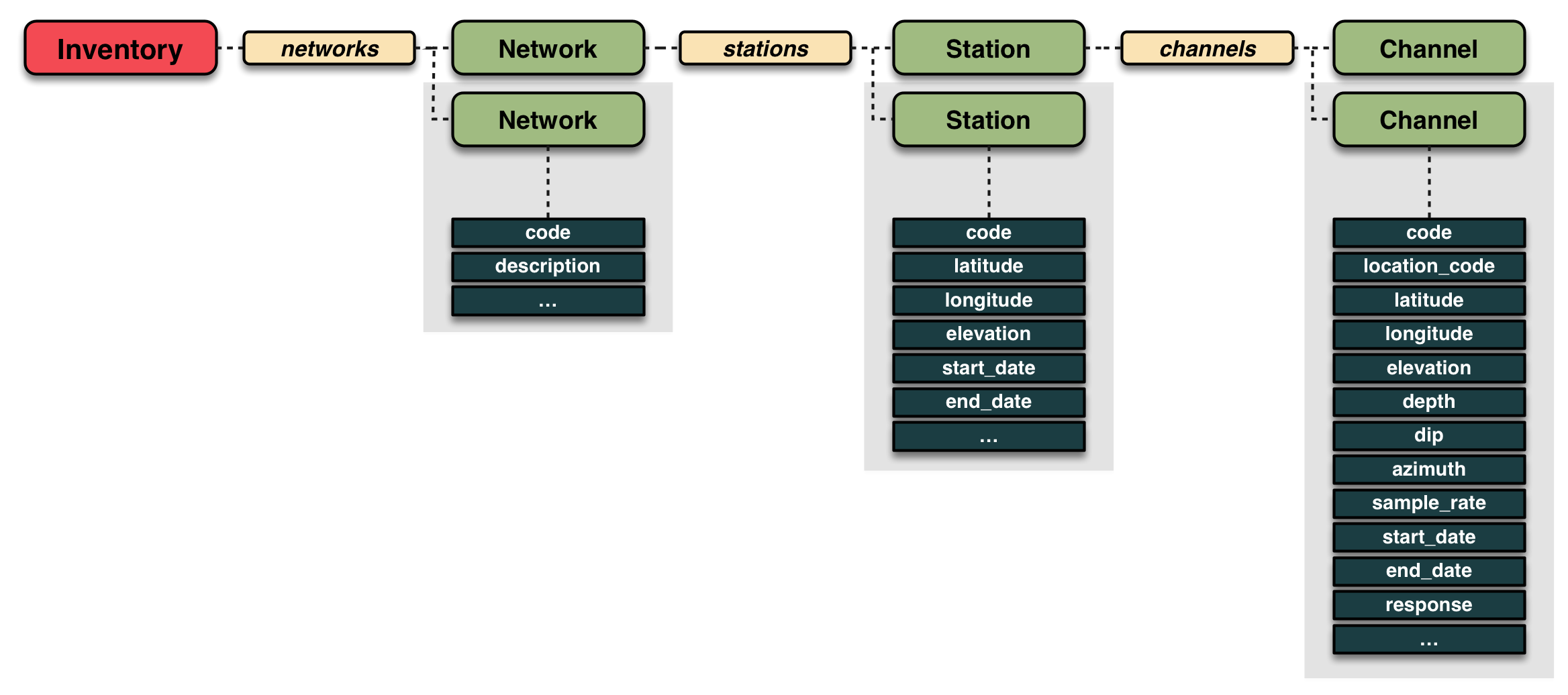
2.1 Membaca StationXML
StationXML dapat dibaca menggunakan fungsi read_inventory karena dalam obspy metadata stasiun diwakili dalam object Inventory, fungsi ini dapat membaca berbagai format (CSS, KML, SACPZ, SHAPEFILE, STATIONTXT, STATIONXML):
from obspy import read_inventory
meta = read_inventory("/content/drive/MyDrive/BMKG_Akselerometer/event-sundastrait-20210321/Dataless/ASJR_manopduatiga_PGN_Seismotek_Inventory_IA.xml")
print(meta)
Inventory created at 2023-07-31T02:07:22.664029Z
	Sending institution: scxml import (ObsPy Inventory)
	Contains:
		Networks (1):
			IA
		Stations (1):
			IA.ASJR (REIS Anyer)
		Channels (3):
			IA.ASJR.00.HNZ, IA.ASJR.00.HNN, IA.ASJR.00.HNE
/usr/local/lib/python3.10/dist-packages/obspy/io/seiscomp/inventory.py:427: UserWarning: Sensor is missing elevation information, using 0.0
  warnings.warn(msg)
Karena file StationXML di atas hanya mewakili 1 stasiun saja maka pada Stations hanya tertulis 1 stasiun saja yaitu REIS Anyer (ASJR). Dalam informasi di atas juga memuat informasi lain seperti waktu pembuatan, jaringan, dan channel.
2.2 Mengakses informasi dalam Inventory
Informasi dalam Inventory atau metadata dapat diakses menggunakan indeks seperti yang dilakukan pada data Stream. Sebagai contoh jika akan mengakses jaringan pertama maka dapat menggunakan indeks 0:
meta[0]
Network IA (BMG-Net, Indonesia (IA-Net))
	Station Count: None/None (Selected/Total)
	1980-01-01T00:00:00.000000Z - --
	Access: open
	Contains:
		Stations (1):
			IA.ASJR (REIS Anyer)
		Channels (3):
			IA.ASJR.00.HNZ, IA.ASJR.00.HNN, IA.ASJR.00.HNE
Demikian pula jika ingin mengakses informasi stasiun pertama pada jaringan pertama maka indeks dapat bertingkat:
meta[0][0]
Station ASJR (REIS Anyer)
	Station Code: ASJR
	Channel Count: None/None (Selected/Total)
	2018-01-02T00:00:00.000000Z -
	Access: closed
	Latitude: -6.06, Longitude: 105.92, Elevation: 0.0 m
	Available Channels:
		ASJR.00.HNZ, ASJR.00.HNN, ASJR.00.HNE
Termasuk mengakses informasi sampai level channel, sebagai contoh disini akan mengambil informasi dari channel ke 2:
meta[0][0][1]
Channel 'HNN', Location '00'
	Time range: 2018-01-02T00:00:00.000000Z - --
	Latitude: -6.06, Longitude: 105.92, Elevation: 0.0 m, Local Depth: 0.0 m
	Azimuth: 0.00 degrees from north, clockwise
	Dip: 0.00 degrees down from horizontal
	Sampling Rate: 100.00 Hz
	Sensor (Description): SM (GFZ:IA1980:G210S/g=0)
	Response information available
Setelah sampai pada tahap ini kita juga masih bisa mengakses sampai informasi yang mendetail, misalkan mengambil nama sensor:
meta[0][0][1].sensor
Equipment:
	Type: SM
	Description: GFZ:IA1980:G210S/g=0
	Manufacturer: Meisei
	Vendor: None
	Model: G210S
	Serial number: None
	Installation date: None
	Removal date: None
	Resource id: Sensor/20181102134034.587314.41
	Calibration Dates:
2.3 Mengakses Informasi Respon Instrumen
Seperti pada 2.2 kita bisa mengambil informasi respon instrumen dengan key response seperti contoh di bawah:
response=meta[0][0][1].response
Termasuk untuk mengeplot respon instrumen:
response.plot(min_freq=1, output="ACC")
No handles with labels found to put in legend.

2.4 Menyimpan Metadata dalam File
Selain membaca metadata, obspy juga memfasilitasi penyimpanan metadata dalam bentuk file dengan Inventory.write dalam berbagai format (CSS, KML, SACPZ, SHAPEFILE, STATIONTXT, STATIONXML), misalkan kita akan menyimpan dalam format SAC Pole and Zero:
meta.write('/content/drive/MyDrive/BMKG_Akselerometer/metadata_baru.pz', format='SACPZ')
Akan muncul file dengan nama metadata_baru.pz dalam file explorer yang bisa dibuka.
3 Melakukan Koreksi Instrumen
Dengan menggunakan metadata stasiun maka kita dapat melakukan koreksi instrumen (dekonvolusi respon instrumen) pada data seismik untuk mendapatkan gerakan tanah sesungguhnya (true ground motion). Proses koreksi instrumen dapat dilakukan dengan bantuan remove_response dari Stream.
3.1 Mendapatkan akselerasi tanah
Akselerasi dapat dipilih dengan memilih ACC pada opsi output:
st_acc = st.copy()
st_acc.remove_response(inventory=meta, output='ACC', plot=True)
3 Trace(s) in Stream:
IA.ASJR.00.HNZ | 2021-03-21T05:56:43.000000Z - 2021-03-21T06:31:43.000000Z | 100.0 Hz, 210001 samples
IA.ASJR.00.HNN | 2021-03-21T05:56:43.000000Z - 2021-03-21T06:31:43.000000Z | 100.0 Hz, 210001 samples
IA.ASJR.00.HNE | 2021-03-21T05:56:43.000000Z - 2021-03-21T06:31:43.000000Z | 100.0 Hz, 210001 samples


Dari hasil di atas terdapat 6 plot, 3 plot dalam domain frekuensi dan 3 plot di kolom sebelahnya dalam domain waktu yang masing-masing mewakili: data mentah (raw), data prapemrosesan (dalam proses diatas tidak dilakukan/None), dan data hasil koreksi (response removed). Pada proses di atas bentuk spektrum bisa terlihat sedikit perbedaan dalam nilai amplitudo ataupun bentuk spektrum (biru) misal di rentang frekuensi rendah. Dari segi bentuk gelombang tidak terlalu terlihat perbedaan tetapi dari nilai amplitudo sudah jauh berbeda.
3.2 Mendapatkan kecepatan tanah
Sama seperti proses pada akselerasi, kita hanya perlu mengganti parameter output menjadi VEL:
st_vel = st.copy()
st_vel.remove_response(inventory=meta, output='VEL', plot=True)
3 Trace(s) in Stream:
IA.ASJR.00.HNZ | 2021-03-21T05:56:43.000000Z - 2021-03-21T06:31:43.000000Z | 100.0 Hz, 210001 samples
IA.ASJR.00.HNN | 2021-03-21T05:56:43.000000Z - 2021-03-21T06:31:43.000000Z | 100.0 Hz, 210001 samples
IA.ASJR.00.HNE | 2021-03-21T05:56:43.000000Z - 2021-03-21T06:31:43.000000Z | 100.0 Hz, 210001 samples


3.2 Mendapatkan simpangan (displacement) tanah
st_disp = st.copy()
st_disp.remove_response(inventory=meta, output='DISP', plot=True)
3 Trace(s) in Stream:
IA.ASJR.00.HNZ | 2021-03-21T05:56:43.000000Z - 2021-03-21T06:31:43.000000Z | 100.0 Hz, 210001 samples
IA.ASJR.00.HNN | 2021-03-21T05:56:43.000000Z - 2021-03-21T06:31:43.000000Z | 100.0 Hz, 210001 samples
IA.ASJR.00.HNE | 2021-03-21T05:56:43.000000Z - 2021-03-21T06:31:43.000000Z | 100.0 Hz, 210001 samples


3.4 Koreksi instrumen lebih lanjut
Tiga proses koreksi instrumen di atas menggunakan parameter yang sudah default, kita dapat melihat parameter apa saja yang dapat dimasukkan dalam proses koreksi instrumen dengan:
help(st[0].remove_response)
Help on method remove_response in module obspy.core.trace:

remove_response(inventory=None, output='VEL', water_level=60, pre_filt=None, zero_mean=True, taper=True, taper_fraction=0.05, plot=False, fig=None, **kwargs) method of obspy.core.trace.Trace instance
    Deconvolve instrument response.

    Uses the adequate :class:`obspy.core.inventory.response.Response`
    from the provided
    :class:`obspy.core.inventory.inventory.Inventory` data. Raises an
    exception if the response is not present.

    Note that there are two ways to prevent overamplification
    while convolving the inverted instrument spectrum: One possibility is
    to specify a water level which represents a clipping of the inverse
    spectrum and limits amplification to a certain maximum cut-off value
    (`water_level` in dB). The other possibility is to taper the waveform
    data in the frequency domain prior to multiplying with the inverse
    spectrum, i.e. perform a pre-filtering in the frequency domain
    (specifying the four corner frequencies of the frequency taper as a
    tuple in `pre_filt`).

    .. note::

        Any additional kwargs will be passed on to
        :meth:`obspy.core.inventory.response.Response.get_evalresp_response`,
        see documentation of that method for further customization (e.g.
        start/stop stage and hiding overall sensitivity mismatch warning).

    .. note::

        Using :meth:`~obspy.core.trace.Trace.remove_response` is equivalent
        to using
        :meth:`~obspy.core.trace.Trace.simulate` with the identical
        response provided as
        a (dataless) SEED or RESP file and when using the same
        `water_level` and `pre_filt` (and options `sacsim=True` and
        `pitsasim=False` which influence very minor details in detrending
        and tapering).

    .. rubric:: Example

    >>> from obspy import read, read_inventory
    >>> st = read()
    >>> tr = st[0].copy()
    >>> inv = read_inventory()
    >>> tr.remove_response(inventory=inv)  # doctest: +ELLIPSIS
    <...Trace object at 0x...>
    >>> tr.plot()  # doctest: +SKIP

    .. plot::

        from obspy import read, read_inventory
        st = read()
        tr = st[0]
        inv = read_inventory()
        tr.remove_response(inventory=inv)
        tr.plot()

    Using the `plot` option it is possible to visualize the individual
    steps during response removal in the frequency domain to check the
    chosen `pre_filt` and `water_level` options to stabilize the
    deconvolution of the inverted instrument response spectrum:

    >>> from obspy import read, read_inventory
    >>> st = read("/path/to/IU_ULN_00_LH1_2015-07-18T02.mseed")
    >>> tr = st[0]
    >>> inv = read_inventory("/path/to/IU_ULN_00_LH1.xml")
    >>> pre_filt = [0.001, 0.005, 45, 50]
    >>> tr.remove_response(inventory=inv, pre_filt=pre_filt, output="DISP",
    ...                    water_level=60, plot=True)  # doctest: +SKIP
    <...Trace object at 0x...>

    .. plot::

        from obspy import read, read_inventory
        st = read("/path/to/IU_ULN_00_LH1_2015-07-18T02.mseed", "MSEED")
        tr = st[0]
        inv = read_inventory("/path/to/IU_ULN_00_LH1.xml", "STATIONXML")
        pre_filt = [0.001, 0.005, 45, 50]
        output = "DISP"
        tr.remove_response(inventory=inv, pre_filt=pre_filt, output=output,
                           water_level=60, plot=True)

    :type inventory: :class:`~obspy.core.inventory.inventory.Inventory`
        or None.
    :param inventory: Station metadata to use in search for adequate
        response. If inventory parameter is not supplied, the response
        has to be attached to the trace with
        :meth:`obspy.core.trace.Trace.attach_response` beforehand.
    :type output: str
    :param output: Output units. One of:

        ``"DISP"``
            displacement, output unit is meters
        ``"VEL"``
            velocity, output unit is meters/second
        ``"ACC"``
            acceleration, output unit is meters/second**2
        ``"DEF"``
            default units, the response is calculated in
            output units/input units (last stage/first stage).
            Useful if the units for a particular type of sensor (e.g., a
            pressure sensor) cannot be converted to displacement, velocity
            or acceleration.

    :type water_level: float
    :param water_level: Water level for deconvolution.
    :type pre_filt: list or tuple(float, float, float, float)
    :param pre_filt: Apply a bandpass filter in frequency domain to the
        data before deconvolution. The list or tuple defines
        the four corner frequencies `(f1, f2, f3, f4)` of a cosine taper
        which is one between `f2` and `f3` and tapers to zero for
        `f1 < f < f2` and `f3 < f < f4`.
    :type zero_mean: bool
    :param zero_mean: If `True`, the mean of the waveform data is
        subtracted in time domain prior to deconvolution.
    :type taper: bool
    :param taper: If `True`, a cosine taper is applied to the waveform data
        in time domain prior to deconvolution.
    :type taper_fraction: float
    :param taper_fraction: Taper fraction of cosine taper to use.
    :type plot: bool or str
    :param plot: If `True`, brings up a plot that illustrates how the
        data are processed in the frequency domain in three steps. First by
        `pre_filt` frequency domain tapering, then by inverting the
        instrument response spectrum with or without `water_level` and
        finally showing data with inverted instrument response multiplied
        on it in frequency domain. It also shows the comparison of
        raw/corrected data in time domain. If a `str` is provided then the
        plot is saved to file (filename must have a valid image suffix
        recognizable by matplotlib e.g. '.png').
Dari petunjuk di atas ada beberapa parameter yang dapat digunakan beserta nilai default: output='VEL',water_level=60, pre_filt=None, zero_mean=True, taper=True, taper_fraction=0.05.
4 Simulasi Gerakan Tanah
Jika proses pada (3) merupakan koreksi instrumen yang sebenarnya adalah dekonnvolusi respon instrumen dari data rekaman untuk mendapatkan gerakan tanah sesungguhnya, maka simulasi adalah proses sebaliknya dimana kita dapat mengonvolusi data gerakan tanah dengan instrumen tertentu. Dengan proses ini kita dapat mensimulasikan bagaimana bentuk rekaman atau gerakan tanah jika direkam di instrumen yang berbeda. Sebagai contoh kita akan di bawah kita akan membalik operasi koreksi instrumen dan mensimulasikan apabila gerakan tanah direkam di instrumen broadband Guralp CMG-6T, 1s-100Hz, 2000 V/m/s dengan datalogger DM-24 Mk3 Fixed Gain, gain 1, 1000 sps, tap id 1, (1000 500 250 125 25 and 5 Hz).
4.1 Melakukan simulasi
Kita akan membalik proses koreksi instrumen yang sebelumnya dilakukan, kali ini data yang sudah dalam bentuk percepatan st_acc akan disimulasikan apabila direkam di stasiun ASJR ke dalam count lagi. Sebelumnya kita konversi respon instrumen dalam bentuk objek Response menjadi objek PAZ yang dikenali fungsi untuk simulasi (simulate). Sayangnya sepertinya belum ada fungsi otomatis untuk ini jadi kita harus melakukan semi manual:
respon_stasiun_ASJR = meta[0][0][0].response.get_paz().__dict__
respon_stasiun_ASJR
{'_normalization_frequency': 1.0,
 '_poles': [(-914.825+0j),
  (-6904.65+0j),
  (-3900.17+0j),
  (-67481.5+0j),
  (-7098.57+0j),
  (-98870.4+0j),
  (-3770.74+0j)],
 '_pz_transfer_function_type': 'LAPLACE (RADIANS/SECOND)',
 '_zeros': [(-628.319+0j), (-12566.4+0j), (-62831.9+0j)],
 'decimation_correction': None,
 'decimation_delay': None,
 'decimation_factor': None,
 'decimation_input_sample_rate': None,
 'decimation_offset': None,
 'description': None,
 'input_units': 'M/S**2',
 'input_units_description': None,
 'name': 'GFZ:IA1980:G210S/g=0',
 'normalization_factor': 8868340000000000.0,
 'output_units': 'V',
 'output_units_description': None,
 'resource_id': None,
 'resource_id2': 'ResponsePAZ/20181102134034.587367.42',
 'stage_gain': 0.193877551,
 'stage_gain_frequency': 1.0,
 'stage_sequence_number': 1}
Untuk keperluan simulasi dibutuhkan poles, zeros, gain (A0 normalization factor), dan sensitivity (overall) sehingga perlu kita sesuaikan:
respon_stasiun_ASJR_formatted = dict()
respon_stasiun_ASJR_formatted['poles'] = respon_stasiun_ASJR['_poles']
respon_stasiun_ASJR_formatted['zeros'] = respon_stasiun_ASJR['_zeros']
respon_stasiun_ASJR_formatted['gain'] = respon_stasiun_ASJR['normalization_factor']
respon_stasiun_ASJR_formatted['sensitivity'] = meta[0][0][0].response.instrument_sensitivity.value #overall sensitivity

respon_stasiun_ASJR_formatted
{'gain': 8868340000000000.0,
 'poles': [(-914.825+0j),
  (-6904.65+0j),
  (-3900.17+0j),
  (-67481.5+0j),
  (-7098.57+0j),
  (-98870.4+0j),
  (-3770.74+0j)],
 'sensitivity': 279620.2663,
 'zeros': [(-628.319+0j), (-12566.4+0j), (-62831.9+0j)]}
Selanjutnya kita simulasikan st_acc:
st_acc_ASJR = st_acc.copy()
st_acc_ASJR.simulate(paz_simulate=respon_stasiun_ASJR_formatted)
st_acc_ASJR.plot()

Kemudian kita bisa bandingkan dengan data asli dalam count (st), dalam plot akan digunakan matplotlib:
import matplotlib.pyplot as plt

fig=plt.figure(figsize=(10,6))

ax=fig.add_subplot(2,1,1)
ax.plot(st_acc_ASJR[0].times(), st_acc_ASJR[0].data, color="blue", alpha=1, linewidth=.5, label="Hasil simulasi")

ax2=fig.add_subplot(2,1,2)
ax2.plot(st[0].times(), st[0].data, color="green", alpha=1, linewidth=1, label="Rekaman asli")

ax.set_ylabel("Count")
ax2.set_ylabel("Count")
ax2.set_xlabel("Waktu [s]")

fig.legend(loc='upper center')
<matplotlib.legend.Legend at 0x7f35746ca090>

Apabila kita jadikan 1 plot dan zoom pada waktu 1020-1040 misalkan:
fig=plt.figure(figsize=(10,3))

ax=fig.add_subplot(1,1,1)
ax.plot(st_acc_ASJR[0].times(), st_acc_ASJR[0].data, color="green", alpha=1, linewidth=1, label="Hasil simulasi")
ax.plot(st[0].times(), st[0].data, color="red", alpha=1, linewidth=1, label="Rekaman asli", linestyle="--")

ax.set_ylabel("Count")
ax.set_xlabel("Waktu [s]")
ax.set_xlim(1020,1040)
ax.set_ylim(-200,200)

ax.legend()
<matplotlib.legend.Legend at 0x7f357220fb90>

Lebih detail lagi:
fig=plt.figure(figsize=(10,3))

ax=fig.add_subplot(1,1,1)
ax.plot(st_acc_ASJR[0].times(), st_acc_ASJR[0].data, color="green", alpha=1, linewidth=2, label="Hasil simulasi")
ax.plot(st[0].times(), st[0].data, color="red", alpha=1, linewidth=2, label="Rekaman asli", linestyle="--")

ax.set_ylabel("Count")
ax.set_xlabel("Waktu [s]")
ax.set_xlim(1026,1028)
ax.set_ylim(-200,200)

ax.legend()
<matplotlib.legend.Legend at 0x7f3571f88590>

4.2 Mengambil respon instrumen dari IRIS Nominal Response Logger melalui obspy
Dalam kasus simulasi pada instrumen lain obspy memberi jembatan untuk mendapatkan respon instrumen tertentu dari IRIS NRL:
from obspy.clients.nrl import NRL
nrl = NRL()
nrl
<ipython-input-3-a98dceb481d9>:2: ObsPyDeprecationWarning:
        DEPRECATED

        Direct access to online NRL is deprecated as it will stop working when
        the original NRLv1 gets taken offline (Spring 2023), please consider
        working locally with a downloaded full copy of the old NRLv1 or new
        NRLv2 following instructions on the
        `NRL landing page <https://ds.iris.edu/ds/nrl/>`_.

  nrl = NRL()
NRL library at https://ds.iris.edu/NRL
  Sensors: 42 manufacturers
    'ASIR', 'CEA-DASE', 'CME (now R-Sensors)', 'Chaparral Physics',
    'DTCC (manuafacturers of SmartSolo)', 'EQMet', 'Eentec', 'GEObit'
    'GEOsig', 'GaiaCode', 'Gem', 'Generic', 'Geo Space/OYO',
    'Geodevice', 'Geotech', 'Guralp', 'HGS Products', 'High Tech',
    'Hyperion', 'IESE', 'Johnson Infrasound', 'Kinemetrics', 'LaHusen'
    'Lennartz', 'Lunitek', 'Magseis Fairfield', 'Metrozet',
    'Nanometrics', 'R-Sensors (previously listed as CME', 'REF TEK',
    'RTClark', 'SARA', 'Seismo Wave', 'SensorNederland',
    'Sercel/Mark Products', 'Silicon Audio', 'SolGeo',
    'Sprengnether (now Eentec)', 'Streckeisen', 'Sunfull', 'TDG',
    'iTem'
  Dataloggers: 30 manufacturers
    'Agecodagis', 'CNSN', 'DAQ Systems (NetDAS)',
    'DTCC (manufacturers of SmartSolo', 'DiGOS/Omnirecs', 'EQMet',
    'Earth Data', 'Eentec', 'GEObit', 'Gem', 'Generic', 'GeoSIG',
    'Geodevice', 'Geotech', 'Guralp', 'Kinemetrics', 'Lunitek',
    'Magseis Fairfield', 'Nanometrics', 'Quanterra', 'R-Sensors',
    'REF TEK', 'SARA', 'STANEO', 'Seismic Source',
    'SeismologyResearchCentre', 'Sercel', 'SolGeo', 'TDG',
    'WorldSensing'
Untuk sensor Guralp:
nrl.sensors['Guralp']
Select the Guralp sensor model (14 items):
  'CMG-1T', 'CMG-3ESP', 'CMG-3ESPC', 'CMG-3T', 'CMG-3T/5T Hybrid',
  'CMG-3TB (borehole)', 'CMG-3v', 'CMG-40T', 'CMG-5', 'CMG-5TC',
  'CMG-6T', 'CMG-6TF', 'CMG-EDU-T', 'Fortis'
Seri CMG-6T:
nrl.sensors['Guralp']['CMG-6T']
Select the natural period (or passband) for this sensor (7 items):
  '10s - 100Hz', '1s - 100Hz', '2s - 100Hz', '30s - 100Hz',
  '40s - 100Hz', '5s - 100Hz', '60s - 100Hz'
Misalkan untuk 1s-100 Hz:
nrl.sensors['Guralp']['CMG-6T']['1s - 100Hz']['2000']
('CMG-6T, 1s-100Hz, 2000 V/m/s',
 'https://ds.iris.edu/NRL/sensors/guralp/RESP.XX.NS070..SHZ.CMG6T.1_100.2000',
 'RESP')
Sensitivitas 2000 V/m/s:
response_cmg6t=nrl.sensors['Guralp']['CMG-6T']['1s - 100Hz']['2000']
response_cmg6t
('CMG-6T, 1s-100Hz, 2000 V/m/s',
 'https://ds.iris.edu/NRL/sensors/guralp/RESP.XX.NS070..SHZ.CMG6T.1_100.2000',
 'RESP')
Respon untuk datalogger digunakan Guralp DM-24 Mk3 Fixed Gain, gain 1, 1000 sps, tap id 1, (1000 500 250 125 25 and 5 Hz):
response_guralp=nrl.dataloggers['Guralp']['CMG-DM24']['Mk3']['Fixed']['1-10']['1']['1000']
response_guralp
('DM-24 Mk3 Fixed Gain, gain 1, 1000 sps, tap id 1, (1000 500 250 125 25 and 5 Hz)',
 'http://ds.iris.edu/NRL/dataloggers/guralp/CMG_DM24/mk3/fixed/RESP.XX.G0143..HHZ.CMG_DM24_MK3_FIX.1..1000')
4.2 Membuat objek Response dari respon instrumen sensor dan datalogger
Setelah kita mendapatkan informasi respon sensor dan datalogger maka kita dapat membuat objek Response yang akan digunakan untuk melakukan simulasi, objek ini mirip seperti metadata Inventory hanya pada Response informasi hanya memuat respon instrumen (Response merupakan bagian dari Inventory)/
respon_instrumen = nrl.get_response(
    sensor_keys=['Guralp','CMG-6T','1s - 100Hz','2000'],
    datalogger_keys=['Guralp','CMG-DM24','Mk3','Fixed','1-10','1','1000'])
respon_instrumen
Channel Response
	From M/S (Velocity in Meters per Second) to COUNTS (Digital Counts)
	Overall Sensitivity: 6.24981e+08 defined at 5.000 Hz
	9 stages:
		Stage 1: PolesZerosResponseStage from M/S to V, gain: 2000
		Stage 2: ResponseStage from V to V, gain: 1
		Stage 3: CoefficientsTypeResponseStage from V to COUNTS, gain: 312500
		Stage 4: CoefficientsTypeResponseStage from COUNTS to COUNTS, gain: 1
		Stage 5: CoefficientsTypeResponseStage from COUNTS to COUNTS, gain: 1
		Stage 6: CoefficientsTypeResponseStage from COUNTS to COUNTS, gain: 1
		Stage 7: CoefficientsTypeResponseStage from COUNTS to COUNTS, gain: 1
		Stage 8: CoefficientsTypeResponseStage from COUNTS to COUNTS, gain: 1
		Stage 9: CoefficientsTypeResponseStage from COUNTS to COUNTS, gain: 1
respon_instrumen.plot(min_freq=0.01)
No handles with labels found to put in legend.

4.3 Melakukan simulasi
Pada obspy masih belum ada fungsi untuk konversi Response menjadi dictionary PAZ yang dibutuhkan pada fungsi simulate sehingga kita harus konversi sedikit manual:
respon_instrumen_paz=respon_instrumen.get_paz().__dict__
respon_instrumen_paz
{'_normalization_frequency': 5.0,
 '_poles': [(-4.4422+4.4422j),
  (-4.4422-4.4422j),
  (-391.96+850.69j),
  (-391.96-850.69j),
  (-471.24+0j),
  (-2199.1+0j)],
 '_pz_transfer_function_type': 'LAPLACE (RADIANS/SECOND)',
 '_zeros': [0j, 0j],
 'decimation_correction': None,
 'decimation_delay': None,
 'decimation_factor': None,
 'decimation_input_sample_rate': None,
 'decimation_offset': None,
 'description': None,
 'input_units': 'M/S',
 'input_units_description': 'Velocity in Meters per Second',
 'name': None,
 'normalization_factor': 911329000000.0,
 'output_units': 'V',
 'output_units_description': 'Volts',
 'resource_id': None,
 'resource_id2': None,
 'stage_gain': 2000.0,
 'stage_gain_frequency': 5.0,
 'stage_sequence_number': 1}
Beberapa key perlu kita sesuaikan dengan kebutuhan simulate:
respon_instrumen_paz['poles'] = respon_instrumen_paz['_poles']
respon_instrumen_paz['zeros'] = respon_instrumen_paz['_zeros']
respon_instrumen_paz['gain'] = respon_instrumen_paz['normalization_factor']
respon_instrumen_paz['sensitivity'] = respon_instrumen.instrument_sensitivity.value #overall sensitivity
respon_instrumen_paz
{'_normalization_frequency': 5.0,
 '_poles': [(-4.4422+4.4422j),
  (-4.4422-4.4422j),
  (-391.96+850.69j),
  (-391.96-850.69j),
  (-471.24+0j),
  (-2199.1+0j)],
 '_pz_transfer_function_type': 'LAPLACE (RADIANS/SECOND)',
 '_zeros': [0j, 0j],
 'decimation_correction': None,
 'decimation_delay': None,
 'decimation_factor': None,
 'decimation_input_sample_rate': None,
 'decimation_offset': None,
 'description': None,
 'gain': 911329000000.0,
 'input_units': 'M/S',
 'input_units_description': 'Velocity in Meters per Second',
 'name': None,
 'normalization_factor': 911329000000.0,
 'output_units': 'V',
 'output_units_description': 'Volts',
 'poles': [(-4.4422+4.4422j),
  (-4.4422-4.4422j),
  (-391.96+850.69j),
  (-391.96-850.69j),
  (-471.24+0j),
  (-2199.1+0j)],
 'resource_id': None,
 'resource_id2': None,
 'sensitivity': 624981223.3355017,
 'stage_gain': 2000.0,
 'stage_gain_frequency': 5.0,
 'stage_sequence_number': 1,
 'zeros': [0j, 0j]}
Melakukan simulasi:
st_vel_cmg6t = st_vel.copy()
st_vel_cmg6t.simulate(paz_simulate=respon_instrumen_paz)
st_vel_cmg6t.plot()

Plot rekaman getaran tanah sesungguhnya (velocity) dari akselerometer ASJR:
st_vel.plot()

5 Latihan
5.1 Membaca data seismik stasiun BLJR
from obspy import read

st=read('')
st+=read('')
st+=read('')
print(st)
3 Trace(s) in Stream:
IA.BLJR.00.HNZ | 2021-03-21T05:56:43.000000Z - 2021-03-21T06:31:43.000000Z | 100.0 Hz, 210001 samples
IA.BLJR.00.HNN | 2021-03-21T05:56:43.000000Z - 2021-03-21T06:31:43.000000Z | 100.0 Hz, 210001 samples
IA.BLJR.00.HNE | 2021-03-21T05:56:43.000000Z - 2021-03-21T06:31:43.000000Z | 100.0 Hz, 210001 samples
5.1 Membaca metadata stasiun BLJR
from obspy import read_inventory
meta = read_inventory("")
print(meta)
Inventory created at 2022-07-15T13:25:33.662082Z
	Sending institution: scxml import (ObsPy Inventory)
	Contains:
		Networks (1):
			IA
		Stations (1):
			IA.BLJR (REIS Bayah)
		Channels (3):
			IA.BLJR.00.HNZ, IA.BLJR.00.HNN, IA.BLJR.00.HNE
5.2 Melakukan koreksi instrumen untuk mendapatkan akselerasi
st_acc = st.copy()
st_acc.remove_response(#isikan disini)
3 Trace(s) in Stream:
IA.BLJR.00.HNZ | 2021-03-21T05:56:43.000000Z - 2021-03-21T06:31:43.000000Z | 100.0 Hz, 210001 samples
IA.BLJR.00.HNN | 2021-03-21T05:56:43.000000Z - 2021-03-21T06:31:43.000000Z | 100.0 Hz, 210001 samples
IA.BLJR.00.HNE | 2021-03-21T05:56:43.000000Z - 2021-03-21T06:31:43.000000Z | 100.0 Hz, 210001 samples


